A mean is a compression. Compressions lose things.
Every summary statistic is a trade. You give up detail and you buy a number you can compare, email and put on a slide. The trade is almost always worth making. The problem is that we rarely ask what we paid for it.
In 1973 the statistician Frank Anscombe published four small datasets to make exactly this point. They were built so that the mean of x, the mean of y, the standard deviation of x, the standard deviation of y, the correlation, and therefore the fitted regression line, come out the same to two decimal places. He then drew them. The four pictures look nothing like each other.
The four datasets come from F. J. Anscombe, Graphs in Statistical Analysis, The American Statistician, 1973.
Half a century on, the lesson is easy to agree with and hard to practise, because the tools that made it possible are working against us. A warehouse query returns a mean. A BI dashboard renders a bar. A model reports an R squared. Each of those is a summary, and each of them will happily describe twelve completely different datasets with the same sentence.
What follows is seven demonstrations, and then a protocol. I built the datasets myself, wrote the code, and put everything in a public repository so you can check every number. Two of the demonstrations use real published data, the 1973 Berkeley admissions records and a global health dataset, because the argument only matters if it survives contact with real mess.
Descriptive statistics are a starting point that feels like a conclusion. If your exploratory analysis stops at the mean, the standard deviation and the correlation, you have not found the story, you have found the shape of the envelope. The job is to open it.
Anscombe's quartet: four regressions, one output
Here are Anscombe's four datasets. Read the table first, the way an analyst with a query and a deadline would read it.
| dataset | mean of x | mean of y | SD of x | SD of y | correlation |
|---|---|---|---|---|---|
| set 1 | 9.00 | 7.50 | 3.16 | 1.94 | 0.82 |
| set 2 | 9.00 | 7.50 | 3.16 | 1.94 | 0.82 |
| set 3 | 9.00 | 7.50 | 3.16 | 1.94 | 0.82 |
| set 4 | 9.00 | 7.50 | 3.16 | 1.94 | 0.82 |
Identical. By every number on the page, this is one dataset reported four times. Now draw it, with the same fitted line on each panel.
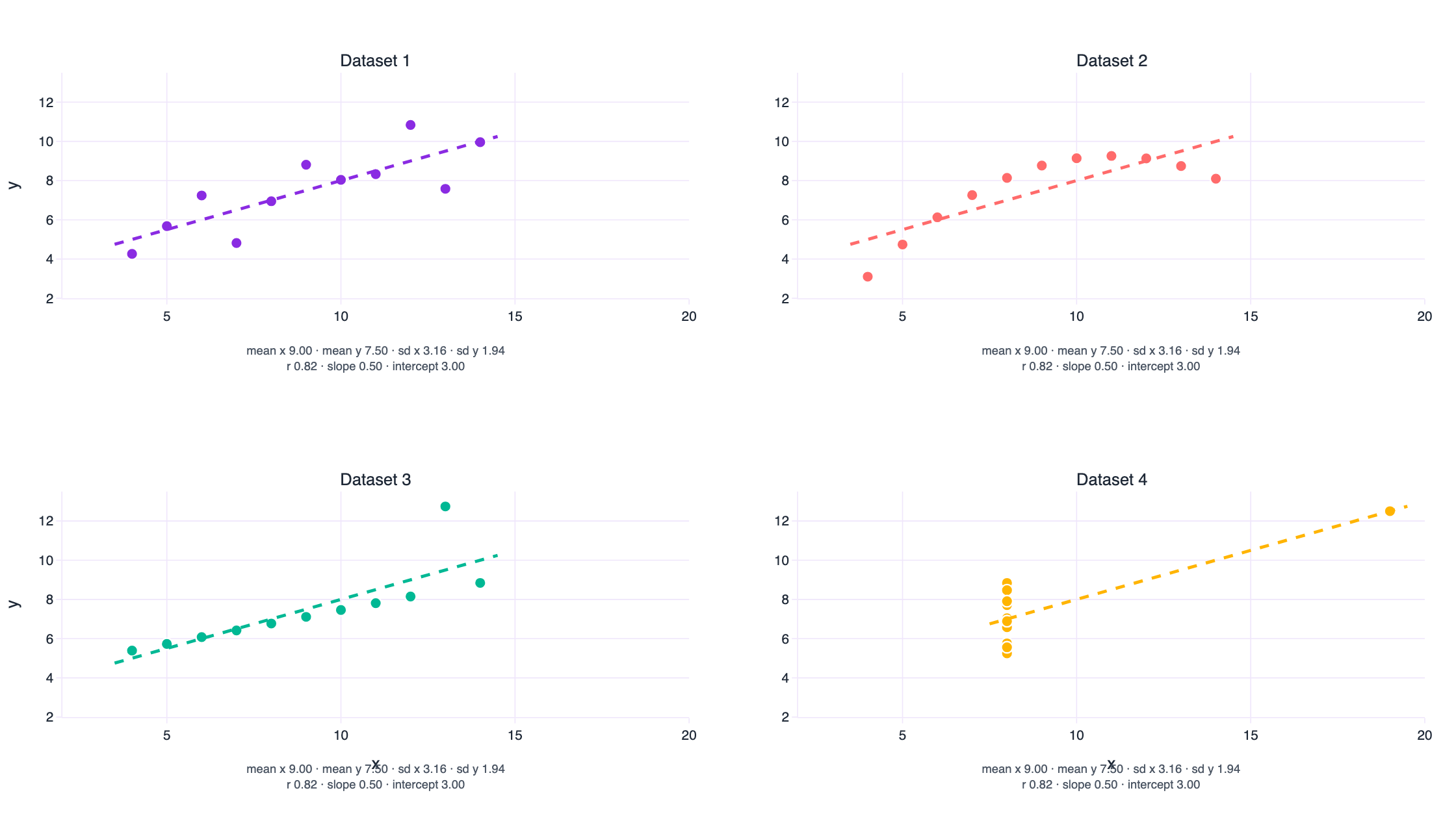
What each panel is telling you
Dataset 1 is the case the regression was invented for. The relationship is straight, the scatter is even, and the line is a fair description of every point on the panel. If all four looked like this, summary statistics would be enough.
Dataset 2 is curved. The points sit on a clean parabola that a straight line can only approximate, so the correlation of 0.82 actually understates a relationship that is nearly deterministic. Add one x squared term and the fit becomes almost exact. Report only the linear correlation and you have just described a strong relationship as a moderate one, and you will probably conclude there is noise in a process that has none.
Dataset 3 is a perfect straight line with a single point pulled out of place. The 10 honest points have a correlation of 1.00. One row drags the reported correlation down to 0.82 and tilts the slope. In a real dataset that row is a data entry error, a different unit of measurement, or a genuinely extreme case. Two of those three need fixing, and the summary statistics cannot tell you which one you have.
Dataset 4 is the trap for anyone who fits before they look. Every x is 8, except for one observation at x = 19. That single point both creates the entire apparent trend and carries a leverage of 1.0, which means the fitted line passes through it exactly. Remove it and the regression is not merely weaker, it is undefined, because x has no variance left. A leverage of 1.0 should be impossible in a dataset you are reporting from. It happens all the time.
If you ran the four regressions in any statistical package, printed the coefficients, the R squared, the standard errors and the p values, and put the printouts on a desk, you would not be able to match the printouts to the pictures. Four different realities, one identical block of output. Anscombe chose the numbers so that the residual standard error, the confidence interval for the slope and the significance test agree as well.
The equality is a property of rounding, and that matters
It is worth being precise about the word “identical”, because statisticians have spent fifty years arguing about it. The four datasets are not arithmetically identical. They agree to two decimal places, which is the precision Anscombe chose for his table.
| dataset | mean of y | SD of y | correlation (r) |
|---|---|---|---|
| set 1 | 7.5009 | 1.9370 | 0.8164 |
| set 2 | 7.5009 | 1.9371 | 0.8162 |
| set 3 | 7.5000 | 1.9359 | 0.8163 |
| set 4 | 7.5009 | 1.9361 | 0.8165 |
The standard deviation of y is 1.9370, 1.9371, 1.9359 and 1.9361. The correlations are 0.8164, 0.8162, 0.8163 and 0.8165. Real differences, hiding two decimal places down.
This is why the next two sections are worth your time. Rounding is a weak form of the trick. If I could build datasets whose statistics are identical to the last binary digit, the objection disappears, and the argument gets sharper: there is no threshold of precision at which the summary statistics start to notice the shape. They never notice. That is what a summary is.
The Datasaurus Dozen, and the method behind it
In 2016 Alberto Cairo published a dataset whose statistics look thoroughly ordinary and whose scatter plot is a dinosaur. His instruction to readers has become the slogan of this whole corner of data visualisation: never trust summary statistics alone; always visualise your data .
A year later, Justin Matejka and George Fitzmaurice at Autodesk Research generalised the idea into a method and published it at CHI 2017 as Same Stats, Different Graphs . Their contribution is not the dinosaur. It is the algorithm: start from any dataset, pick a point, nudge it, keep the nudge if the mean, the standard deviation and the correlation stay inside tolerance, and bias the nudges towards a target shape so the cloud walks towards a picture you chose. They add simulated annealing so the walk does not get stuck in local optima, and they run it until a blob of random numbers has become a circle, a star, an x, three vertical lines.
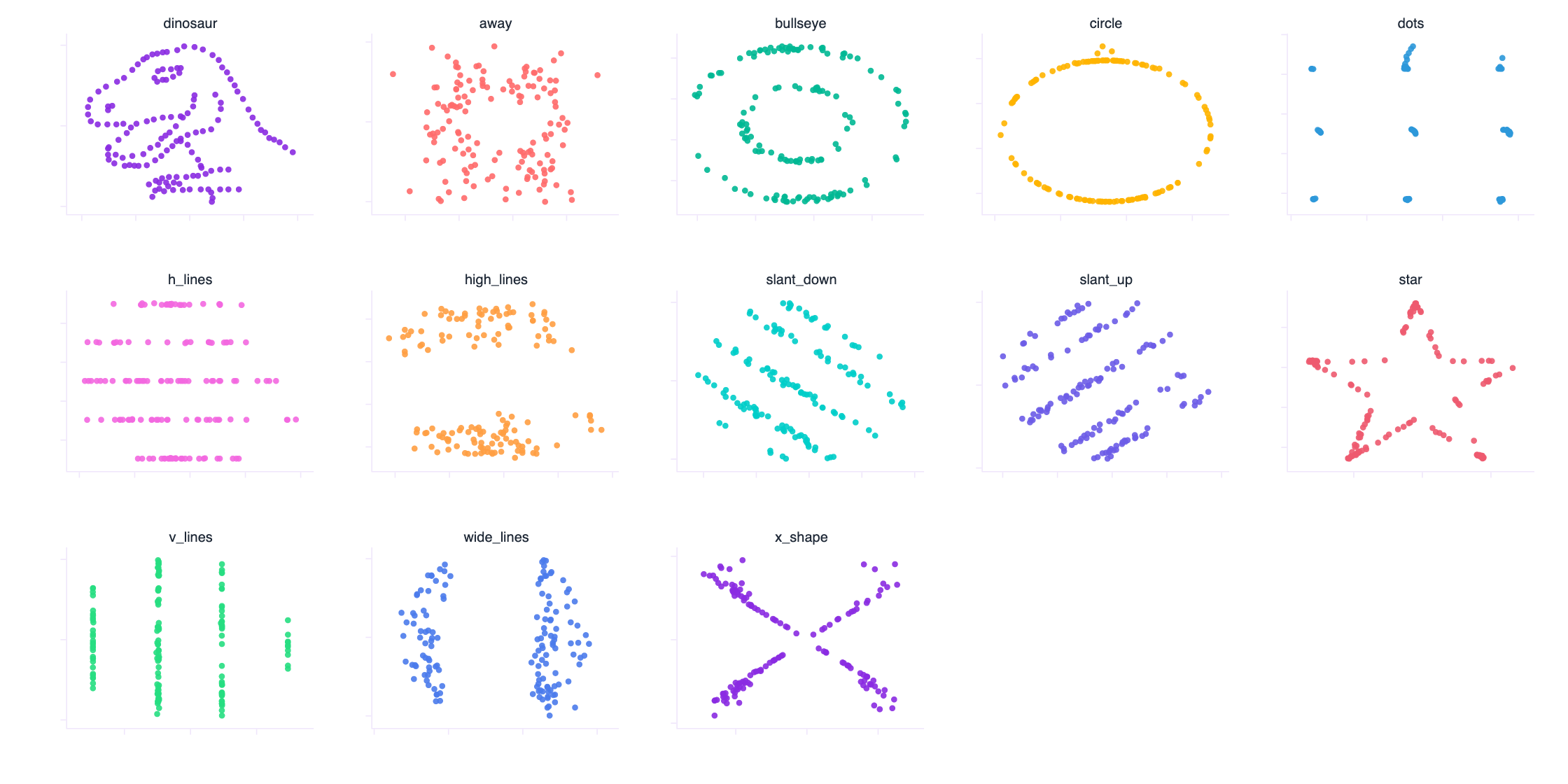
Thirteen panels, thirteen datasets, one summary. The paper's datasets agree to two decimal places, which is plenty to make the argument in a keynote. I wanted to know whether the agreement could be exact rather than close. It can, and it takes four lines of linear algebra rather than two hundred thousand iterations of simulated annealing.
Twelve datasets, statistics identical to fifteen decimal places
Here is the whole trick. Take any cloud of points. Standardise both coordinates so they have mean zero and standard deviation one. The correlation of two standardised variables is the cosine of the angle between them, so if you want a specific correlation, you do not need to search for one: you rotate.
u = (x - mean(x)) / sd(x)            # mean 0, sd 1
v = (y - mean(y)) / sd(y)            # mean 0, sd 1
e = v - (u . v / n) * u              # the part of v perpendicular to u
w = e / sd(e)                        # unit vector, still perpendicular to u

v* = r * u + sqrt(1 - r^2) * w       # corr(u, v*) is now exactly r
x' = m1 + s1 * u                     # mean m1, sd s1, exactly
y' = m2 + s2 * v*                    # mean m2, sd s2, exactly
The affine step fixes the means and the standard deviations because it is arithmetic rather than optimisation. The orthogonal step fixes the correlation because a correlation is a cosine and the two components are at right angles. Nothing in this procedure looks at the shape of the cloud, which is why the shape is free to be anything at all.
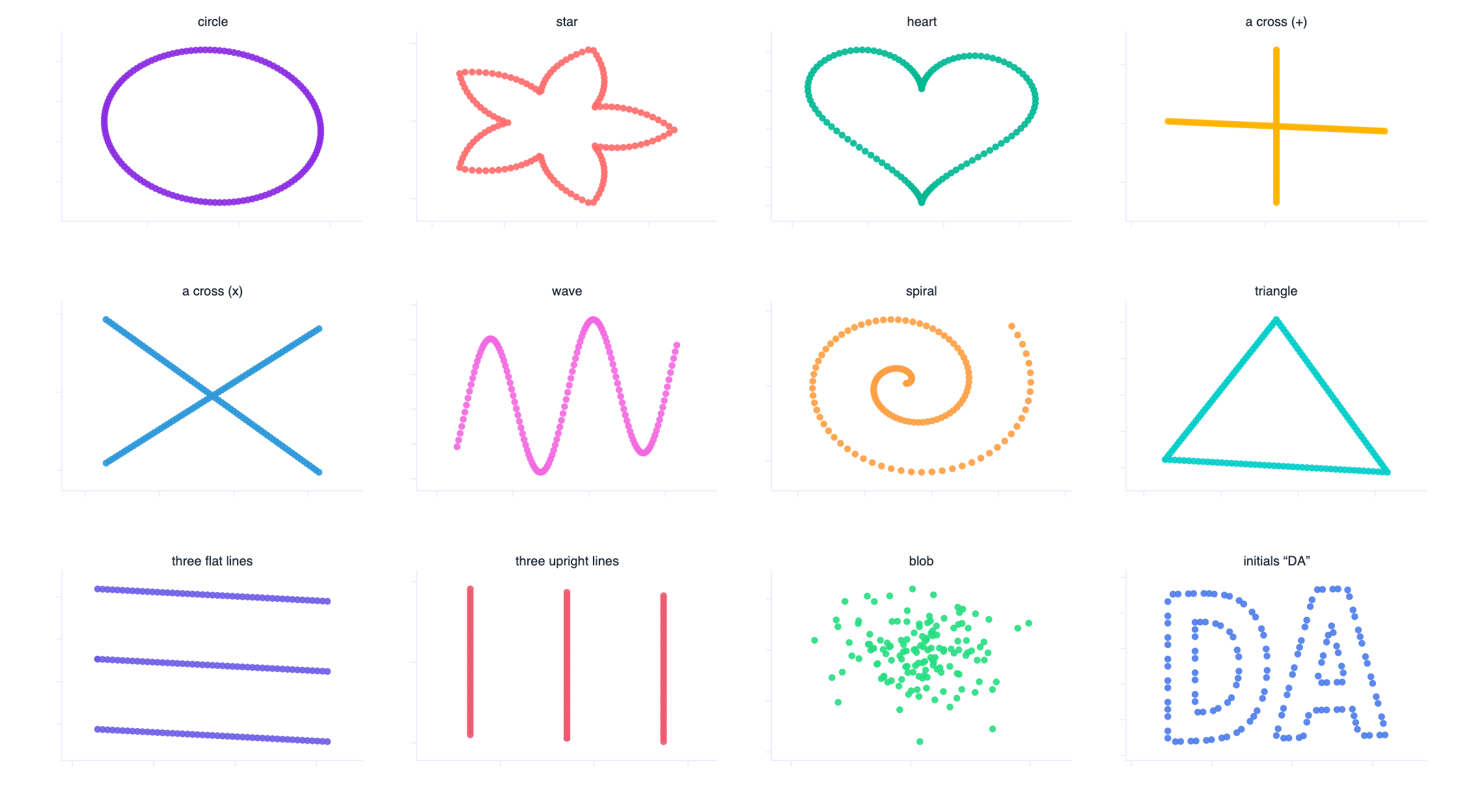
The table below is the verification. Twelve rows, ten decimal places, no argument.
| shape | mean of x | mean of y | SD of x | SD of y | correlation |
|---|---|---|---|---|---|
| circle | 54.2600000000 | 47.8300000000 | 16.7600000000 | 26.9300000000 | -0.0641000000 |
| star | 54.2600000000 | 47.8300000000 | 16.7600000000 | 26.9300000000 | -0.0641000000 |
| heart | 54.2600000000 | 47.8300000000 | 16.7600000000 | 26.9300000000 | -0.0641000000 |
| plus | 54.2600000000 | 47.8300000000 | 16.7600000000 | 26.9300000000 | -0.0641000000 |
| x_shape | 54.2600000000 | 47.8300000000 | 16.7600000000 | 26.9300000000 | -0.0641000000 |
| wave | 54.2600000000 | 47.8300000000 | 16.7600000000 | 26.9300000000 | -0.0641000000 |
| spiral | 54.2600000000 | 47.8300000000 | 16.7600000000 | 26.9300000000 | -0.0641000000 |
| triangle | 54.2600000000 | 47.8300000000 | 16.7600000000 | 26.9300000000 | -0.0641000000 |
| h_lines | 54.2600000000 | 47.8300000000 | 16.7600000000 | 26.9300000000 | -0.0641000000 |
| v_lines | 54.2600000000 | 47.8300000000 | 16.7600000000 | 26.9300000000 | -0.0641000000 |
| blob | 54.2600000000 | 47.8300000000 | 16.7600000000 | 26.9300000000 | -0.0641000000 |
| letters_DA | 54.2600000000 | 47.8300000000 | 16.7600000000 | 26.9300000000 | -0.0641000000 |
The largest disagreement between any two of those rows, across all five statistics, is 1.1 × 10⁻¹⁴. That is floating point arithmetic running out of room, not a statistical difference. You could train a model on any one of these twelve datasets and print a metric, and the metric would be the same to every digit the machine can hold, while the thing you are modelling is a spiral in one case and a heart in another.
Notice what the trick does not preserve. Skewness, kurtosis, the number of modes and every nonlinear statistic are free to differ, and they do, wildly. So the summary is not merely incomplete in an abstract sense. It is incomplete in a way that is structural: the statistics that survive the transformation are exactly the ones that cannot see shape, and the statistics that see shape are exactly the ones nobody puts in the table.
Three honest caveats, because this is a demonstration, not a proof of anything universal. These twelve datasets are synthetic and they were built to make a point, so treat the shapes as an illustration of the arithmetic rather than as evidence about anyone's data. Higher moments are not preserved, which is the whole idea. And the transformation is not a substitute for the Autodesk method: their perturbation approach generalises to any statistic you can compute, while mine works because the mean, the standard deviation and the correlation are exactly the statistics an affine-plus-rotation map can control. That is also why they are the statistics that get quoted.
Everything from here on uses either real data or datasets whose distributions are constructed to mirror shapes you meet in operational work.
The mean and the standard deviation do not describe a shape
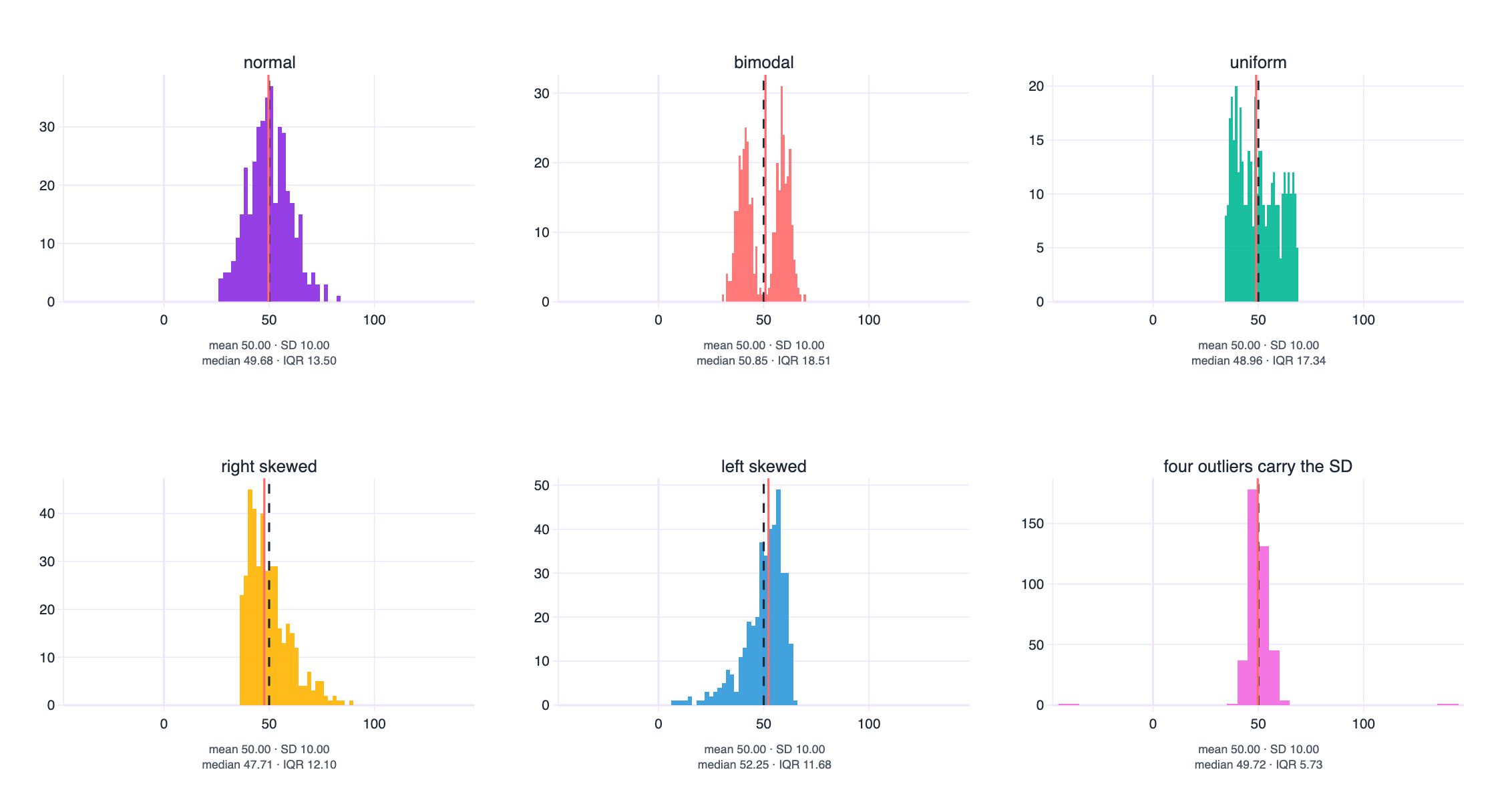
Set the shape question aside for a moment and keep only two numbers, the pair that ends up in almost every report ever written. Six distributions below all have a mean of 50.00 and a standard deviation of 10.00, exactly, by construction.
| distribution | mean | SD | median | IQR (Q3-Q1) | min | max | skewness |
|---|---|---|---|---|---|---|---|
| normal | 50.00 | 10.00 | 49.68 | 13.50 | 26.6 | 83.7 | +0.14 |
| bimodal | 50.00 | 10.00 | 50.85 | 18.51 | 30.5 | 69.2 | -0.03 |
| right_skewed | 50.00 | 10.00 | 47.71 | 12.10 | 36.1 | 88.3 | +1.10 |
| left_skewed | 50.00 | 10.00 | 52.25 | 11.68 | 6.6 | 64.2 | -1.47 |
| uniform | 50.00 | 10.00 | 48.96 | 17.34 | 34.2 | 68.4 | +0.23 |
| outlier_driven | 50.00 | 10.00 | 49.72 | 5.73 | -44.4 | 144.7 | +0.05 |
Same two headline numbers, and the story underneath is different in every panel.
The bimodal pair of humps is the clearest case. The mean of 50 sits in a gap where almost no observation lives. That is not a subtle statistical objection, it is a direct contradiction: the number you are reporting describes an outcome that does not happen. Two humps almost always means two populations, two shifts, two products, two customer segments, and the right next step is to find the variable that separates them rather than to report their average.
The skewed panels show why the mean drifts away from anything a person would recognise as typical. In the right skewed case the median sits at 47.71 while the mean is at 50, because a modest number of large values pull the mean up. In real operational data, service times, claim amounts, waiting lists and call durations are skewed in this direction, and the mean is routinely read as “the typical case” when it is nothing of the sort.
The last panel is the one I would put in front of any analyst who reports a standard deviation without a plot. Four rows out of four hundred sit far out on the tails. Those four rows alone manufacture the entire standard deviation of 10.00. Remove them and the interquartile range collapses to 5.73 against 13.50 for the normal case with the same standard deviation. The headline number is not describing the spread of your data. It is describing four records.
The mean and the standard deviation are a complete description of one distribution, the normal one, and a partial description of every other. They are least trustworthy exactly where real business data lives: skewed, bounded, spiky, contaminated, or quietly bimodal. Report the median and the interquartile range with them, report n, and report the minimum and the maximum. Then show the histogram, because a reader can absorb a shape in a second and a standard deviation never.
The boxplot mirage
The usual fix for a misleading mean is a boxplot, and it is a real improvement: five numbers instead of two, resistant to outliers, and instantly comparable across groups. It also runs into the same wall, one step further along. Six datasets below share a single five-number summary.
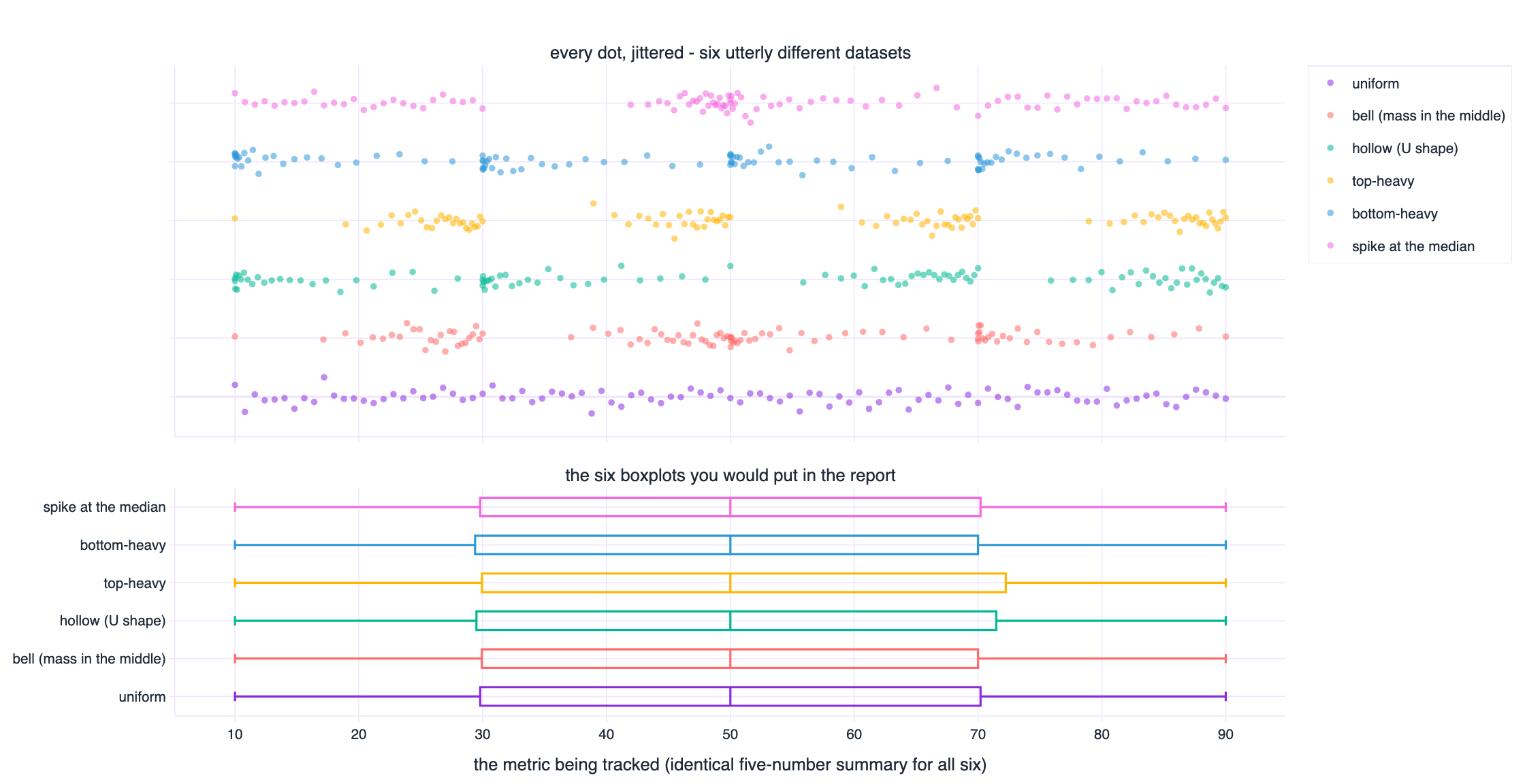
| dataset | min | Q1 | median | Q3 | max | IQR | mean | SD |
|---|---|---|---|---|---|---|---|---|
| uniform | 10.00 | 30.00 | 50.00 | 70.00 | 90.00 | 40.00 | 50.00 | 23.32 |
| hollow (U shape) | 10.00 | 30.00 | 50.00 | 70.00 | 90.00 | 40.00 | 50.00 | 27.06 |
| bell (mass in the middle) | 10.00 | 30.00 | 50.00 | 70.00 | 90.00 | 40.00 | 50.17 | 19.11 |
| top-heavy | 10.00 | 30.00 | 50.00 | 70.00 | 90.00 | 40.00 | 55.83 | 22.91 |
| bottom-heavy | 10.00 | 30.00 | 50.00 | 70.00 | 90.00 | 40.00 | 44.82 | 23.29 |
| spike at the median | 10.00 | 30.00 | 50.00 | 70.00 | 90.00 | 40.00 | 50.82 | 22.37 |
The five-number summary is identical by construction, and the mean still wanders from 44.82 to 55.83 while the standard deviation moves from 19.11 to 27.06. One dataset is a uniform spread. One crowds towards the middle. One is hollow, with the mass pushed into the tails. One is top heavy, one bottom heavy, one is a spike at the median with thin tails on either side.
If you have ever presented a wall of boxplots over a time series, this is the failure mode to worry about. The dashed box does not move, so nothing in the report moves, while the thing you are actually tracking has changed from a bell into a U. The Autodesk authors demonstrate the same effect over time, seven distributions that shift shape year after year while their boxplots stay frozen, and use it to argue for strip plots and violin plots that show density rather than quartiles.
Why this is an operations problem, not a statistical one
Consider a service desk whose response times become bimodal because a new team is handling a new ticket type. The median gets faster and the interquartile range gets narrower, both of which look like improvement on a boxplot, while an entire second population of slow jobs grows into the tail. The people experiencing that second population are the ones most likely to leave, and their experience is invisible in exactly the chart most teams use to monitor experience.
Tukey designed the boxplot to compare medians and flag outliers, and it does that job well. It was never a density plot. If the shape of the distribution is what your decision depends on, draw something that shows shape.
Overlay the individual points on the boxplot whenever the number of observations is small enough for dots to be readable, which in most reporting situations it is. And plot the distribution of the same metric at two points in time side by side, not just its median, because the question “did the centre move” and the question “did the shape move” are different questions with different answers.
Correlation is a number about a line, not about a relationship
Five datasets below all have a Pearson correlation of 0.7000, exactly. They are not five variations on the same theme. They are a line, a curve, a step, a single-point accident, and a mostly random cloud with a late flourish.
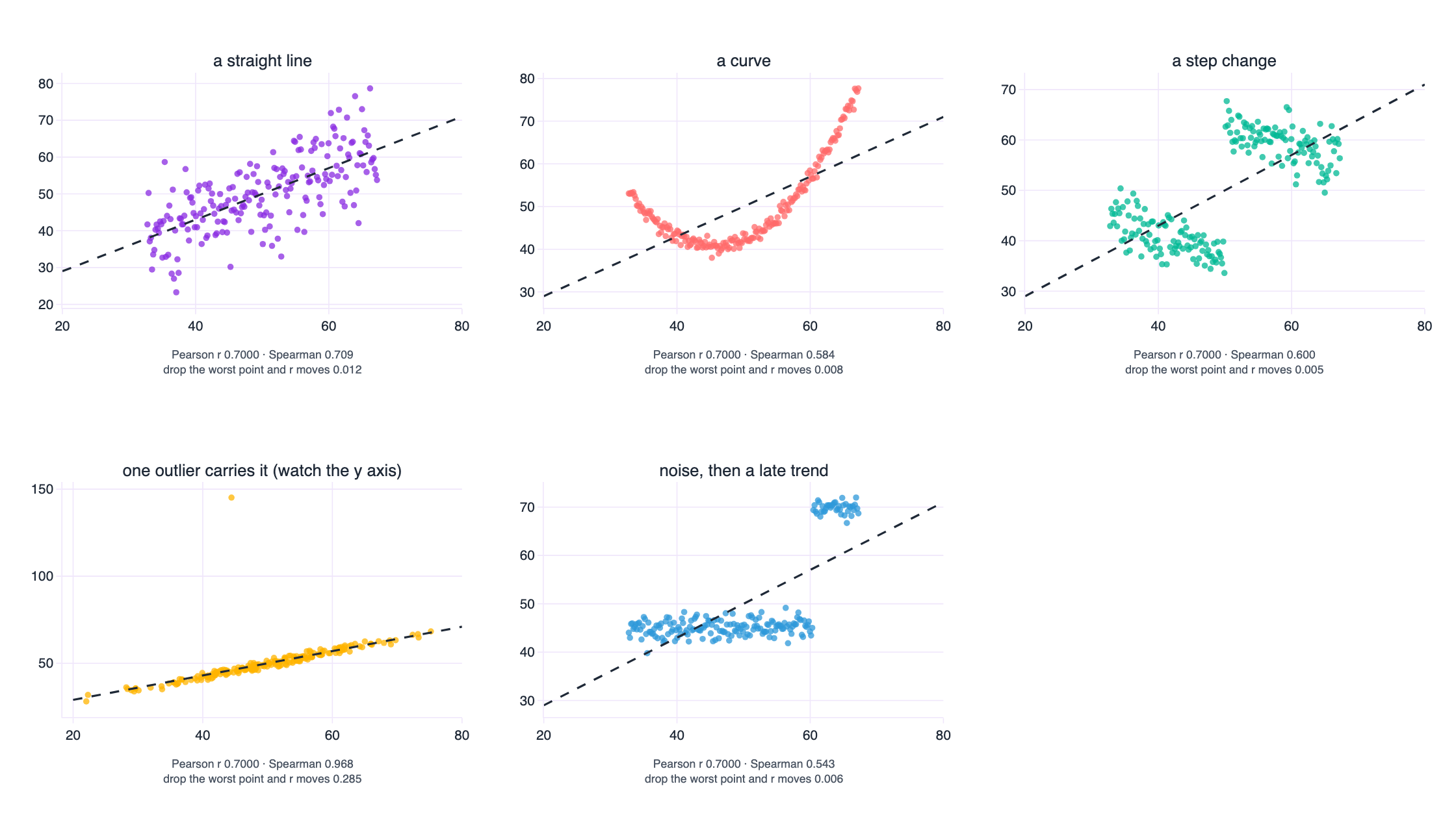
| dataset | Pearson r | Spearman rho | r moves this much if you delete one point |
|---|---|---|---|
| linear | 0.7000 | 0.709 | 0.012 |
| curved (quadratic) | 0.7000 | 0.584 | 0.008 |
| step change | 0.7000 | 0.600 | 0.005 |
| one outlier flips it | 0.7000 | 0.968 | 0.285 |
| wall of noise + trend | 0.7000 | 0.543 | 0.006 |
The second panel is the most common real-world case: a genuine relationship that happens to be curved. Correlations are a summary of the linear component of a relationship and nothing else, so a strong curve is reported as a moderate line. If you fit a straight line through it and then reason about the residuals as noise, you are treating structure as error, and your confidence intervals will be wrong in a way that no amount of extra data will fix.
The third panel is the one that catches experienced people, because both variables are genuinely related, up to a threshold, and then the relationship changes. Correlation has no way to represent a change in regime, so it averages two regimes into one number that describes neither.
The fourth panel is the influence problem in its purest form. Remove the single most consequential point and the correlation moves by 0.285. That is a dataset where the headline number is being held up by one row, and where any conclusion about the population is really a conclusion about one observation.
The extreme case: a perfect relationship with a correlation of zero
If all of that still feels like a matter of degree, here is the limiting case. Take every point on a circle. The relationship between x and y is perfect and deterministic: give me x and I can tell you y, up to a sign. The correlation is zero.
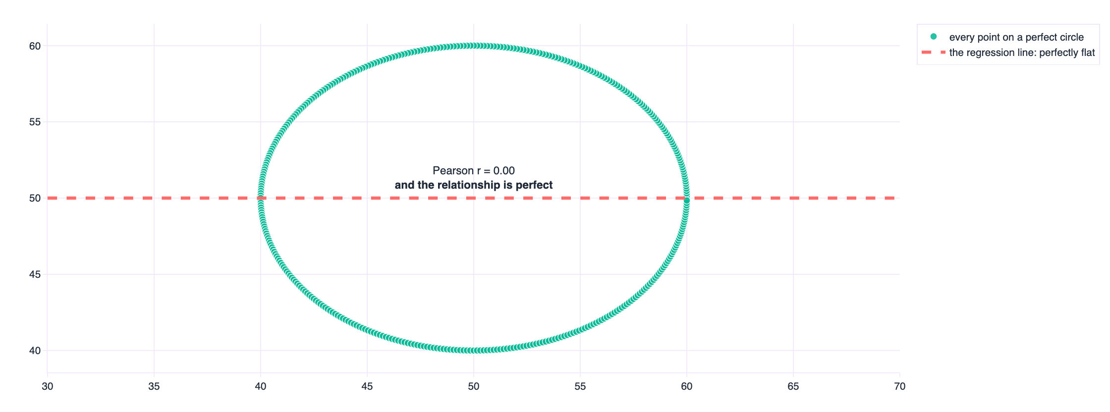
The circle is a cartoon, but the family it belongs to is not. A U-shaped relationship, an X, a sine wave, a heteroscedastic fan where the correlation holds in the middle and fails at the edges, and any cloud with two clusters at opposite corners all produce correlations near zero while containing strong structure. A low correlation is evidence about linear association. It is not evidence of independence, and it is not evidence that nothing is there.
The pooled correlation that measures the wrong thing
Here is the same problem in real data, and it is the reason I put the penguins in.
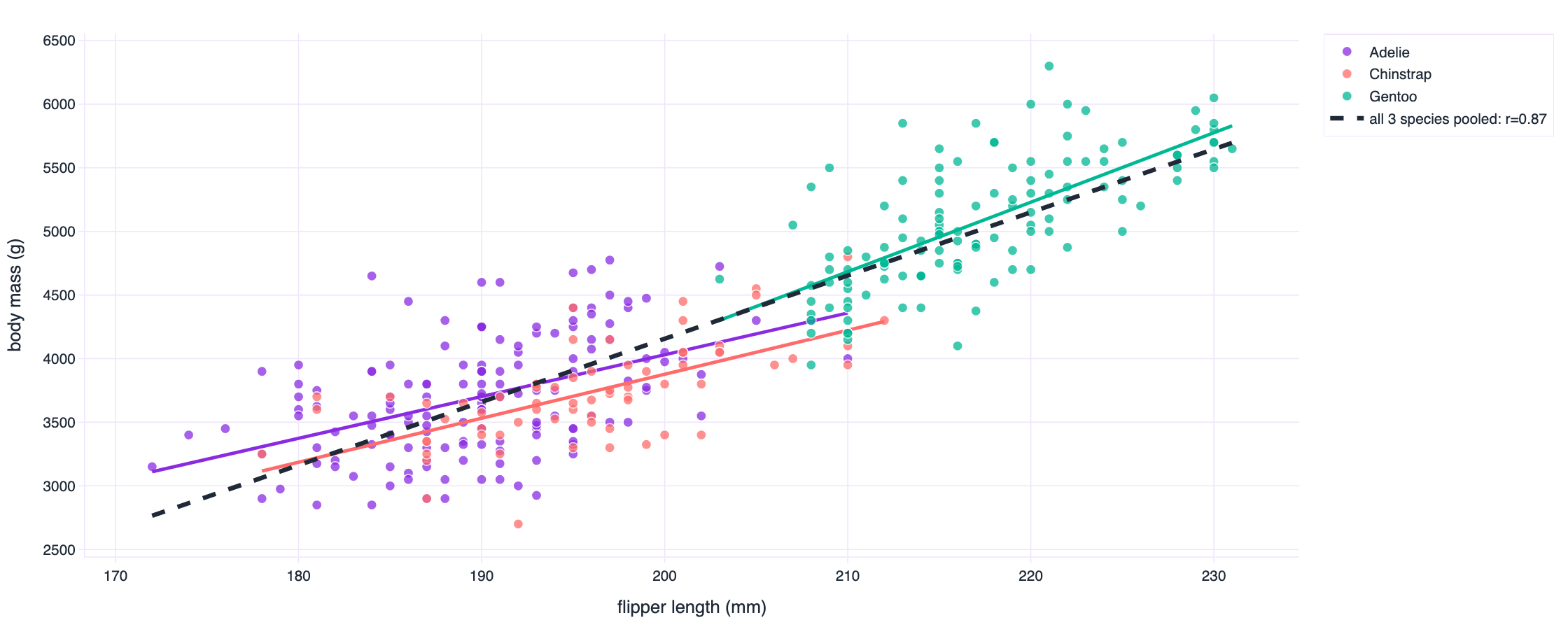
| population | correlation between flipper length and body mass | n |
|---|---|---|
| all three species pooled | 0.871 | 342 |
| Adelie | 0.468 | 151 |
| Chinstrap | 0.642 | 68 |
| Gentoo | 0.703 | 123 |
Pooled, the correlation is 0.871, close to the kind of number somebody quotes as a strong relationship. Inside each species it falls to 0.468, 0.642 and 0.703. The pooled figure is mostly a measurement of how different a Gentoo is from an Adelie, dressed up as a measurement of how flipper length relates to mass. Both statements are true, and only one of them is useful for the question a biologist is usually asking.
The correlation, n, and the scatter plot. A rank correlation alongside it, because Spearman survives curvature and outliers in ways Pearson does not. The influence of the most consequential few points. And the correlation computed separately within each group you know about, because that last number is the one that usually changes the decision.
Simpson's paradox: the number reverses when you remember the groups
Every example so far has been about a statistic failing to describe a single population well. This one is worse, because the statistic reverses. It is not vague, it is wrong in the direction of the conclusion.
In 1973 the University of California at Berkeley was accused of discriminating against women in graduate admissions, on the basis of exactly the kind of aggregate number a report would contain. Peter Bickel, Eugene Hammel and John O'Connell reanalysed the applications, department by department, and published what they found in Science in 1975. Their table, for the six largest departments, is reproduced here.
| department | men applied | men admitted | men rate | women applied | women admitted | women rate | who was admitted more often |
|---|---|---|---|---|---|---|---|
| A | 825 | 512 | 62.1% | 108 | 89 | 82.4% | women higher |
| B | 560 | 353 | 63.0% | 25 | 17 | 68.0% | women higher |
| C | 325 | 120 | 36.9% | 593 | 202 | 34.1% | men higher |
| D | 417 | 138 | 33.1% | 375 | 131 | 34.9% | women higher |
| E | 191 | 53 | 27.7% | 393 | 94 | 23.9% | men higher |
| F | 373 | 22 | 5.9% | 341 | 24 | 7.0% | women higher |
| ALL | 2,691 | 1,198 | 44.5% | 1,835 | 557 | 30.4% | men higher |
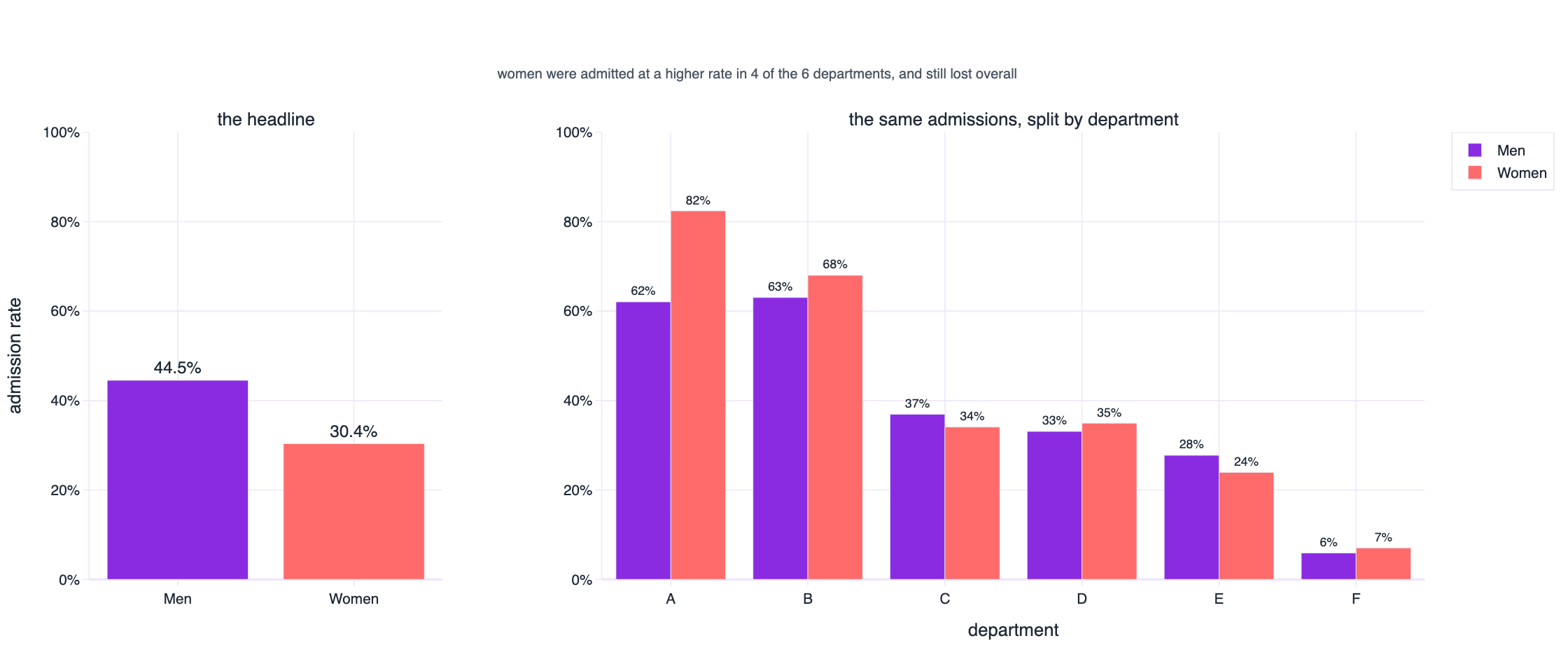
Overall, 44.5 per cent of the men who applied were admitted against 30.4 per cent of the women. Inside the departments, women were admitted at a higher rate in four of the six. Both of those sentences are arithmetic facts about the same 4,526 applications.
The mechanism is the reason this is not a curiosity. Women applied in far greater numbers to the departments that admit almost nobody, and men applied in greater numbers to the departments that admit most applicants. When the two groups have different sizes and the groups have different admission rates, pooling them creates a mixture, and a mixture can run in the opposite direction to every one of its parts. The aggregate was not just imprecise. It pointed at the wrong culprit, and the correction required knowing which groups existed.
The same reversal in a dataset you would meet on a Tuesday
Berkeley is history, so here is a synthetic version of the ordinary case: three schools, hours of revision against exam score. Within each school more revision means a better score. Pool all the students and the correlation flips negative.
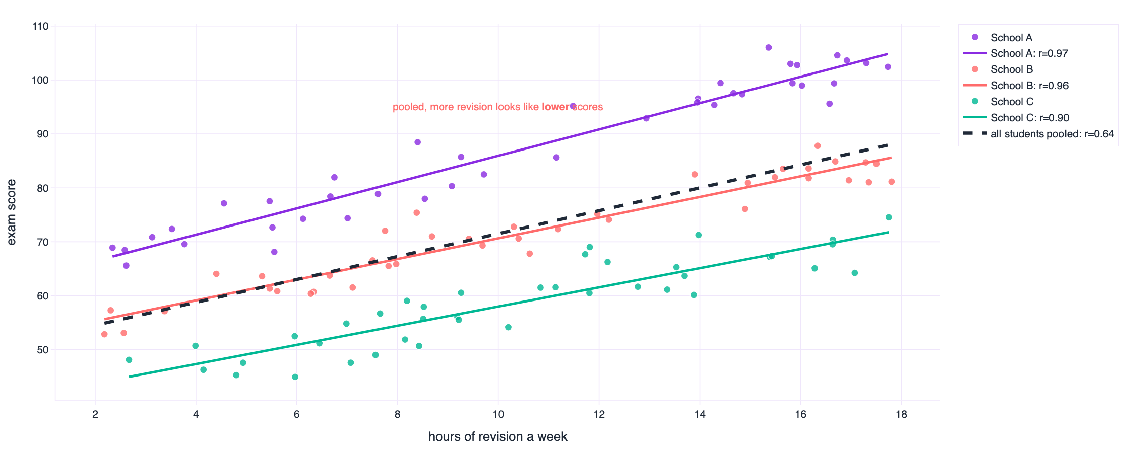
The pooled correlation is 0.636 and it points the wrong way; within schools it runs between 0.898 and 0.969. Nobody is confused about which number matters once they see the picture, and nobody would have seen it from the pooled output.
Real data does the same thing without being constructed for the purpose. Log GDP per person and life expectancy correlate at 0.81 across 142 countries. Inside Africa the same two variables correlate at 0.45. The pooled number is a statement about the difference between continents, not about the relationship between money and years inside a continent. Both are interesting. Mixing them up is how a report ends up saying something nobody can act on.
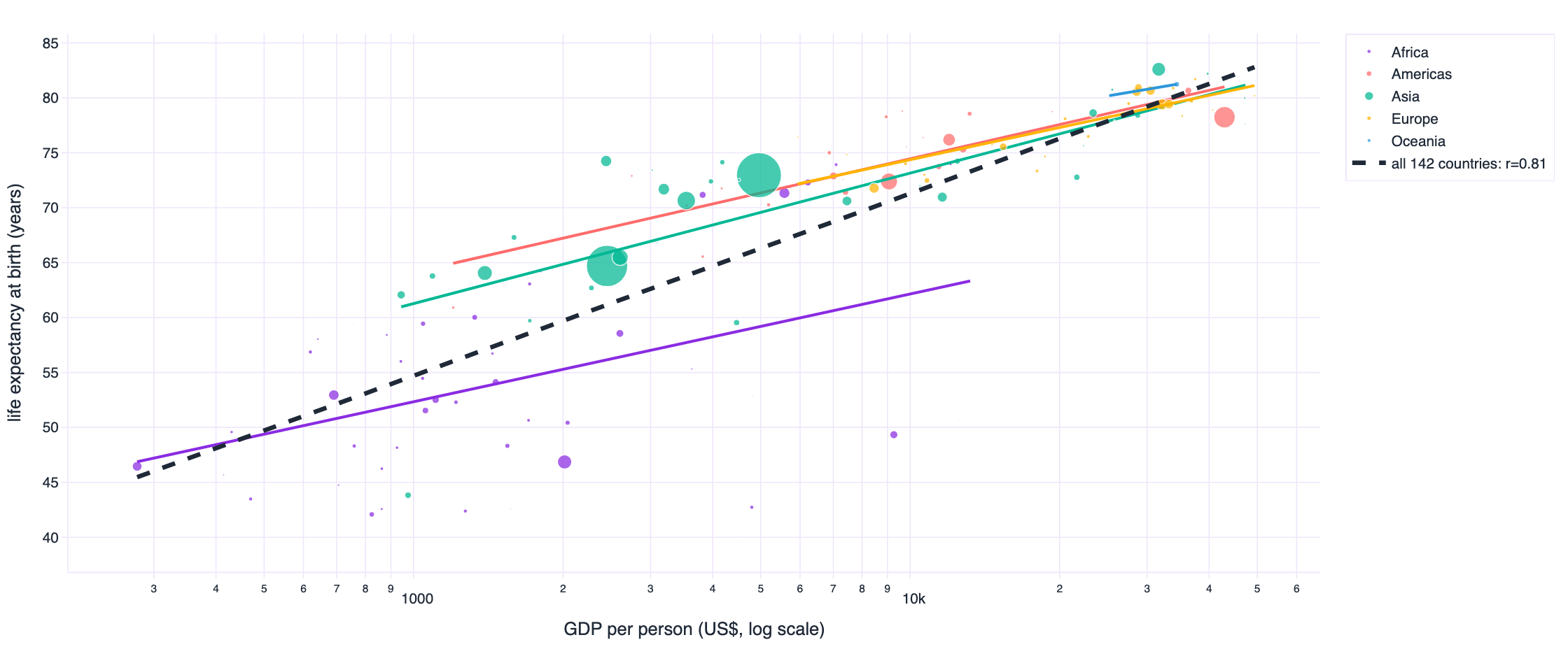
| population | correlation between log GDP per person and life expectancy |
|---|---|
| all countries | 0.809 |
| within Africa | 0.452 |
| within Americas | 0.780 |
| within Asia | 0.800 |
| within Europe | 0.836 |
| within Oceania | 1.000 |
Compare two hospitals on readmission rates without adjusting for case mix and the hospital that treats the sickest patients looks the worst. Compare two service centres on average handling time without separating case types and the centre with harder work looks inefficient. Report a single unemployment rate while the composition of the labour force changes and the aggregate can rise while every group's rate falls. In each case the pooled number is arithmetically correct, easy to compute, and the wrong number for the decision in front of you.
How to catch it before someone else does
Ask what decides which group an observation lands in. If that thing also plausibly affects the outcome, you have a candidate for a reversal, and the groups are almost certainly unequal in size. Then plot the groups, always, even when the pooled chart looks convincing, and compute the statistic both pooled and within. When they disagree, the within-group number answers the causal question and the pooled number answers a question about composition. Say which one you are reporting, in the chart title if necessary.
What the job actually is
None of the seven demonstrations is a surprising piece of mathematics. They are surprises about how much we trust the first number we compute, and that trust is the part of the job that separates a report from an analysis.
Descriptive statistics answer the question “what is the value of this quantity”. They cannot answer “what does this quantity mean”, because meaning depends on shape, on groups and on the decision being made. Someone has to look. In most organisations that someone is the analyst, and the reason it matters is that the summary statistics will never ask for a second look on their own. They are always confident.
- Draw the distribution before you quote its mean. A histogram takes ten seconds and settles most of the questions in this article.
- Never report a mean without n and its median. Two numbers turn a fragment into a description.
- Add the quartiles, the minimum and the maximum. The interquartile range survives the outliers that inflate the standard deviation.
- Ask whether the mean is a place anyone actually is. If it lands in a gap between two humps, the mean describes nobody and the two humps are the story.
- For any relationship, plot first and compute second. Then report the correlation with n, the rank correlation, and the influence of the most consequential observations.
- Look for curvature, thresholds and clusters. A quadratic term, a regime change or two blobs will each defeat a correlation in a different way.
- Stratify before you pool. If you know a variable that affects both group membership and the outcome, compute the statistic inside the groups as well as across them.
- When a trend is reported, ask whether the shape moved, not just the centre. Growing tails and new humps are operational signals and they are invisible in a median.
- Test the robustness of the headline. Recompute without the top and bottom percentile. If the conclusion changes, your conclusion was about the extremes, so say so.
- Keep the picture next to the number. A dashboard showing a mean should carry a link to its distribution, and a report should show both.
The awkward part, in plain terms
This is judgement work rather than software work, and it is where domain knowledge earns its place. Nothing in a query engine will tell you that the response time distribution has turned bimodal because a new ticket type arrived, or that the admissions aggregate mixes departments with wildly different capacity. A statistician with no context can compute every number in this article correctly and still miss every single one of the seven points, because the seven points are all questions about the world rather than about the arithmetic.
The EDA habit worth building is a short reflexive pause between getting a number and reporting a number. Why is it that size. What would make it wrong. What is the picture behind it. What changes in my recommendation if the picture is not what I assumed. Nine times out of ten the pause costs a minute and changes nothing. The tenth time it changes the decision, and nobody notices the nine, which is why the habit is hard to acquire and worth keeping.
import pandas as pd
import plotly.express as px

df = pd.read_csv("data/same_mean_sd_twins.csv")

# 1. the summary you were about to report
summary = df.groupby("dataset")["value"].agg(["mean", "std", "median", "count"])

# 2. the five numbers that spare you an argument
quartiles = df.groupby("dataset")["value"].describe(percentiles=[.25, .5, .75])

# 3. the check nobody does: is this distribution even one distribution?
fig = px.histogram(df, x="value", facet_col="dataset", facet_col_wrap=3,
                   nbins=45, color="dataset", height=560)
fig.show()

# 4. and for a relationship, picture before coefficient
scatter = px.scatter(df_xy, x="x", y="y", trendline="ols", color="group")
scatter.show()
Three lines of pandas and two charts. That is the entire intervention. The reason it does not happen is not that it is difficult, it is that the summary arrives first and looks finished.
Every number here is generated from a public repository
The datasets, the generators and the figures were built with Python, NumPy, pandas and Plotly. Nothing in this article was typed by hand: the tables are generated from the same JSON the figures read, so if a number and a chart ever disagree, the build would break.
File in data/ | What it demonstrates | Rows |
|---|---|---|
| anscombe_quartet.csv | The 1973 original, four sets, identical to two decimal places | 44 |
| same_stats_shapes.csv | Twelve shapes, statistics identical to 15 decimal places | 1,704 |
| datasaurus_dozen.csv | The published Datasaurus Dozen, thirteen shapes | 1,846 |
| same_mean_sd_twins.csv | Six distributions, mean 50.00, standard deviation 10.00 | 2,400 |
| same_boxplot.csv | Six datasets, one identical five-number summary | 606 |
| same_correlation.csv | Five relationships, one correlation of 0.7000 | 1,000 |
| circle_r_zero.csv | A perfect relationship with a correlation of zero | 400 |
| simpson_berkeley_1973.csv | Real admissions data, aggregate reverses by department | 12 |
| simpson_schools.csv | Revision and scores, positive within schools, negative pooled | 120 |
| gapminder_2007.csv | Real GDP and life expectancy, ecological fallacy | 142 |
| penguins.csv | Real measurement data, pooled versus within-species correlation | 342 |
Running it
git clone https://github.com/AbdoDameen/same-stats-different-graphs.git
cd same-stats-different-graphs

uv venv --python 3.11 .venv
uv pip install --python .venv/bin/python numpy pandas scipy plotly kaleido matplotlib

.venv/bin/python scripts/01_make_datasets.py   # builds data/ and verifies every claim
.venv/bin/python scripts/02_build_figures.py   # builds the figures and the tables
.venv/bin/python scripts/03_build_article.py   # assembles this page
01_make_datasets.py prints its own verification: the maximum spread across the twelve identical datasets, the five-number summaries, every correlation. If the arithmetic in this article were wrong, the script would say so before I could publish it.
Attribution
The Anscombe quartet and the Datasaurus Dozen are redistributed here for study, from the published sources cited below. The Berkeley admissions table is the six-department table from Bickel, Hammel and O'Connell (1975). The Gapminder and Palmer Station penguin data are the public datasets of those projects. Everything else was generated by the scripts in this repository from seeded random draws, which means you can rebuild each of them to the last digit.
Code is released under the MIT licence. Datasets are released under CC BY 4.0, with attribution to the original authors above. If you reuse the article itself, a link back is appreciated.
The seven demonstrations in this article are all cases where a true number produced a false impression. None of them required bad faith, sloppy work or a hidden agenda. They required only that someone report the summary and stop. That is the whole failure mode, and it is available to all of us on any Tuesday afternoon, with any dataset, and it is cheap to avoid.
Sources
- Anscombe, F. J. (1973). Graphs in Statistical Analysis. The American Statistician, 27(1), 17–21. The four datasets, the identical regressions and the argument for looking.
- Matejka, J. and Fitzmaurice, G. (2017). Same Stats, Different Graphs: Generating Datasets with Varied Appearance and Identical Statistics through Simulated Annealing. Proceedings of CHI 2017. DOI 10.1145/3025453.3025912. The Datasaurus Dozen, the boxplot and violin examples, and the perturbation method.
- Autodesk Research (2017). Same Stats, Different Graphs, project page with datasets, animations and source code. research.autodesk.com/publications/same-stats-different-graphs.
- Cairo, A. (2016). Download the Datasaurus: Never trust summary statistics alone; always visualize your data. The Functional Art. The original dinosaur.
- Bickel, P. J., Hammel, E. A. and O'Connell, J. W. (1975). Sex Bias in Graduate Admissions: Data from Berkeley. Science, 187(4175), 398–404. The source of the admissions table.
- Simpson, E. H. (1951). The Interpretation of Interaction in Contingency Tables. Journal of the Royal Statistical Society, Series B, 13(2), 238–241. The result now called Simpson's paradox.
- Tukey, J. W. (1977). Exploratory Data Analysis. Addison-Wesley. The origin of the boxplot and of the habit of looking before calculating.
- Tufte, E. R. (1983). The Visual Display of Quantitative Information. Graphics Press. On what a chart can carry that a table cannot.
- Gapminder Foundation. GDP per capita and life expectancy by country, 2007. gapminder.org/data.
- Gorman, K. B., Williams, T. D. and Fraser, W. R. (2014). Ecological Sexual Dimorphism and Environmental Variability within a Community of Antarctic Penguins. PLoS ONE, 9(3). Palmer Station LTER penguin measurements.
How to cite this article
Dameen, A. (2026). Same Numbers, Different Stories.
Dameen Analytics. https://github.com/AbdoDameen/same-stats-different-graphs